Easy Optimization With Evolutionary Strategies

I recently read Ferenc Huszár's blog post summarizing recent research on how evolutionary strategies can be used in place of gradient descent or back-propagation. That research focuses on how evolutionary strategies for reinforcement learning get the same results as back-propagation, but the computation is more parallelizable and therefore faster.

This method caught my attention because it's incredibly flexible, and can be used to optimize many sort of problems beyond finding this optimal parameters for a machine learning model.

I decided to have some fun with it, and see whether evolutionary strategies can help us interpret machine learning models. What I'm doing here differs from the previous work in two ways.

1) Differentiable vs. Non-Differentiable Optimization

Most recent discussions of evolutionary strategies have focused on optimizing the parameters of a neural network to minimize loss - which should be a differentiable function. In that setting either evolutionary strategies or back-propagation should reach a good final outcome (since evolutionary strategies are simply finding the gradient through trial-and-error), and the debate is therefore mostly a question of computational resources.

But for problems with non-differentiable objective functions, gradient descent and back-propagation are difficult and evolutionary strategies seem to me to be an easy and effective solution.

For example: let's say you have a machine learning model that classifies images of hand-written digits as one of the numbers 0-9. We might want to know what the model is looking for when it is deciding whether an image contains the number 5. This could be useful for debugging the model and understanding the ways in which it is likely to perform badly.

If your model is based on regression, you can just use the model's coefficients to find out what your model considers to be an ideal version of the number 5. If your model is a multi-layer neural network, you can use back-propagation to do the same thing - which works because the surface of outcomes (i.e. the probability that a given image is the number 5) is differentiable.

But what if your model is a random forest? The surface of outcomes is not easily differentiable. Evolutionary strategies can solve this problem.

2) Optimizing Model Parameters vs. Model Input

As mentioned above - I'm not using evolutionary strategies to find the optimal parameters for a model, I'm trying to figure out which image will most convince the model that it is an image of the number 5, or any digit 0-9. The beauty of evolutionary strategies is that it can be used to optimize any sort of black box function that takes in an input and outputs a score. It doesn't matter too much whether the function takes in model parameters and outputs log-loss, or takes in an image and outputs a probability.

Demonstration

The algorithm is very simple - in plain English, you:

1. Propose a guess for an image that your model will score highly (for a given digit 0-9).

2. Generate n_children sets of random noise around that guess, each of which looks like a new image. We can call these the "child" images.

3. Use the model to evaluate how the child images increase or decrease the score.

4. Propose a new guess that's in the direction of the better child images and away from the worse ones (a bit more technically - estimate the gradient and move in that direction).

5. Repeat #'s 2-4 until you're happy with the results.

That is what the below code does - it creates a random forest to classify images of handwriting as digits, and uses evolutionary strategies to figure out what the model considers to be the most ideal version of the digits 0-9

import numpy as np
from sklearn.ensemble import RandomForestClassifier
from sklearn import datasets
import matplotlib.pyplot as plt

def find_best_img(score_fn, epochs, n_children, sd, lr, max_score=1):
    """Find an image that gets the highest score on a given model
    Assumes that images are all 8*8 pixels with values in the 0-16 range
    """
    img = np.random.random(64) * 16
    for _ in range(epochs):
        noise = [np.random.normal(0, sd, 64) for _ in range(n_children)]
        child_scores = np.array([score_fn(img + n) for n in noise])
        child_stdev = np.std(child_scores)
        if child_stdev == 0:
            break # we've reached a plateau
        # normalize the scores
        child_scores -= np.mean(child_scores)
        child_scores /= child_stdev
        # see the paper and Huszar's blog post for the math behind this
        gradient = np.mean([n * s for n,s in zip(noise, child_scores)],
                           axis=0) / sd
        img += lr * gradient
        img = np.minimum(np.maximum(img, 0), 16) #constrain pixel values
        img_score = score_fn(img)
        if img_score >= max_score:
            break # no reason to continue

    return img, img_score

def score_function(mod, ix):
    def _scorer(x):
        return mod.predict_proba(x.reshape(1, -1)).flatten()[ix]
    return _scorer

digits = datasets.load_digits()
rf = RandomForestClassifier(criterion="entropy", n_estimators=100,
                            min_samples_leaf=5)
# We don't need a holdout - but we should still care about overfitting, an
# overfitted model is less likely to help us find useful or interesting images.
np.random.seed(5)
rf.fit(digits.data, digits.target)

# Now let's find out what images maximally activate our random forest
best_images = {}
for target in range(10):
    best_images[target] = find_best_img(
        score_function(rf, target),
        epochs=300,
        n_children=25,
        sd=3,
        lr=0.75
    )

We can run this same process for any type of supervised learning model, the code to do this is on my Github page. This method is convenient because we don't have to change any aspect of it for different types of models, we can just treat them as black box scoring machines. Other ways of finding the same information would require model-specific methods.

Below are the ideal images for each digit for 4 different models. The y-axis labels denote the digit and the model score (in the 0-1 range) that it converged on. It's no surprise that different models differ on what they consider to be the ideal version of a given digit. It also shouldn't be too surprising that so many of these images barely look like digits - the models process and understand the data differently than we do, and they only see the 5,620 training images.

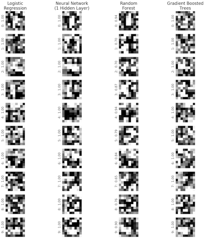
Ideal Digits 0-9, By Model (y-axis text denotes digit: model_score)

We can also create a simple ensemble model that averages the scores of the other 4 models, and find the optimal image for that model (note that this is different than finding the average of the other 4 optimal images). The ensemble model's images look much closer to what we recognize as digits.

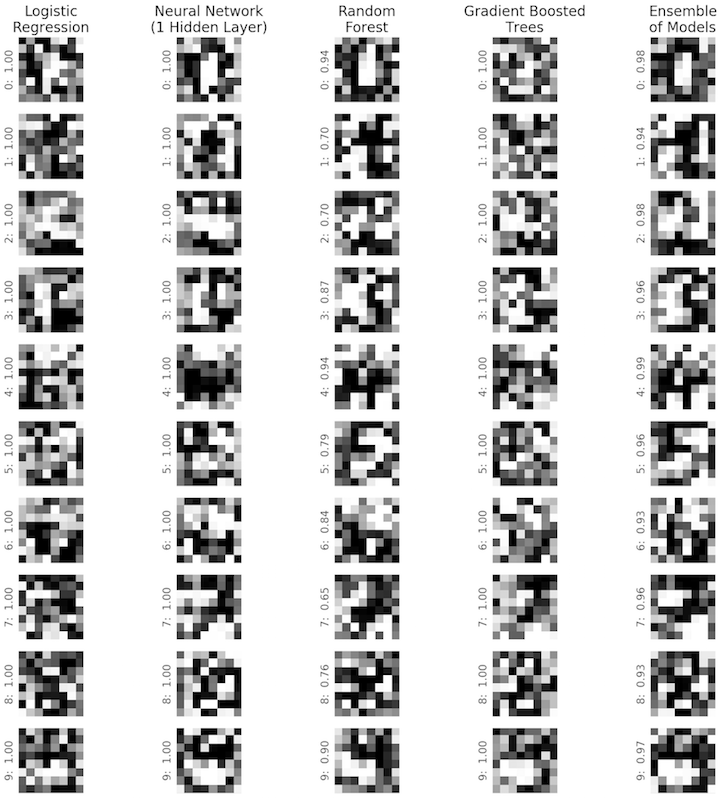
Ideal Digits 0-9, By Model + Ensemble